Demographic Inference
fastcxt’s pairwise TMRCA predictions provide a direct window into historical effective population size. By binning predicted coalescence times into time windows, we compute inverse instantaneous coalescence rates (IICR) — a non-parametric proxy for Ne(t).
This approach follows the same methodology used in cxt’s demography tutorial, adapted for fastcxt’s continuous output format.
Theory
Given a sample of pairwise TMRCAs, the coalescence rate in time window \([t_i, t_{i+1})\) is estimated as:
where \(c_i\) is the count of pairs coalescing in the window, \(S_i\) is the number of surviving (not yet coalesced) lineage pairs at the start of the window, and \(\Delta t_i = t_{i+1} - t_i\).
The IICR is then:
Under a panmictic Wright-Fisher model, IICR equals the effective population size. Under structured populations or with inversions, IICR reflects the pairwise coalescence landscape — deviations from the true Ne reveal population structure, admixture, or selection.
Code example
import numpy as np

def coalescence_rates(tmrcas_generations, time_windows):
    """Compute piecewise coalescence rates from TMRCA samples.

    Parameters
    ----------
    tmrcas_generations : array
        Coalescence times in generations (NOT log-scale).
    time_windows : array
        Bin edges, e.g. np.logspace(2, 7, 41) with [0] = 0.

    Returns
    -------
    rates : array of coalescence rates per window.
    """
    counts, _ = np.histogram(tmrcas_generations, bins=time_windows)
    total = len(tmrcas_generations)
    cum = np.cumsum(counts)
    surviving = total - np.concatenate([[0], cum[:-1]])
    widths = np.diff(time_windows)
    rates = np.where(
        (surviving > 0) & (widths > 0),
        (counts / surviving) / widths,
        0.0,
    )
    return rates

# From fastcxt predictions
means = np.load("means.npz")["means"]
tmrcas_gen = np.exp(means.flatten())  # log -> generations

time_windows = np.logspace(2, 7, 41)
time_windows[0] = 0.0
rates = coalescence_rates(tmrcas_gen, time_windows)
iicr = 1.0 / (2.0 * rates)  # proxy for Ne

time_mids = np.sqrt(time_windows[:-1] * time_windows[1:])
Comparing to stdpopsim
The stdpopsim catalog includes a demographic model for A. gambiae Gabon
(GabonAg1000G_1A17), estimated from the Ag1000G Phase 1 data using
stairway plot. We overlay this reference on our IICR estimates:
import stdpopsim

species = stdpopsim.get_species("AnoGam")
demogr = species.get_demographic_model("GabonAg1000G_1A17")
pop_name = demogr.model.populations[0].name

fine_grid = np.logspace(0, 7, 1000)
coalrate, _ = demogr.model.debug().coalescence_rate_trajectory(
    lineages={pop_name: 2}, steps=fine_grid,
)
ref_iicr = 1.0 / (2.0 * coalrate)
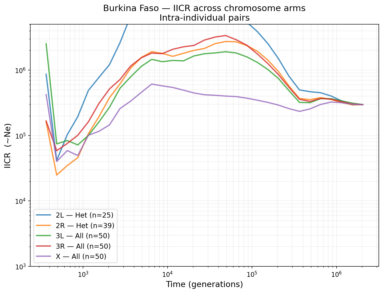
Burkina Faso IICR from intra-individual pairs across all chromosome arms, compared to the stdpopsim Gabon reference (dashed black). Chromosomes 3L and 3R (no inversions) provide the cleanest demographic signal.
Karyotype effects on IICR
Inversions distort the IICR because they suppress recombination between standard and inverted arrangements. For heterozygous individuals, the two haplotypes inside the inversion have very deep coalescence, inflating the IICR at intermediate time scales:
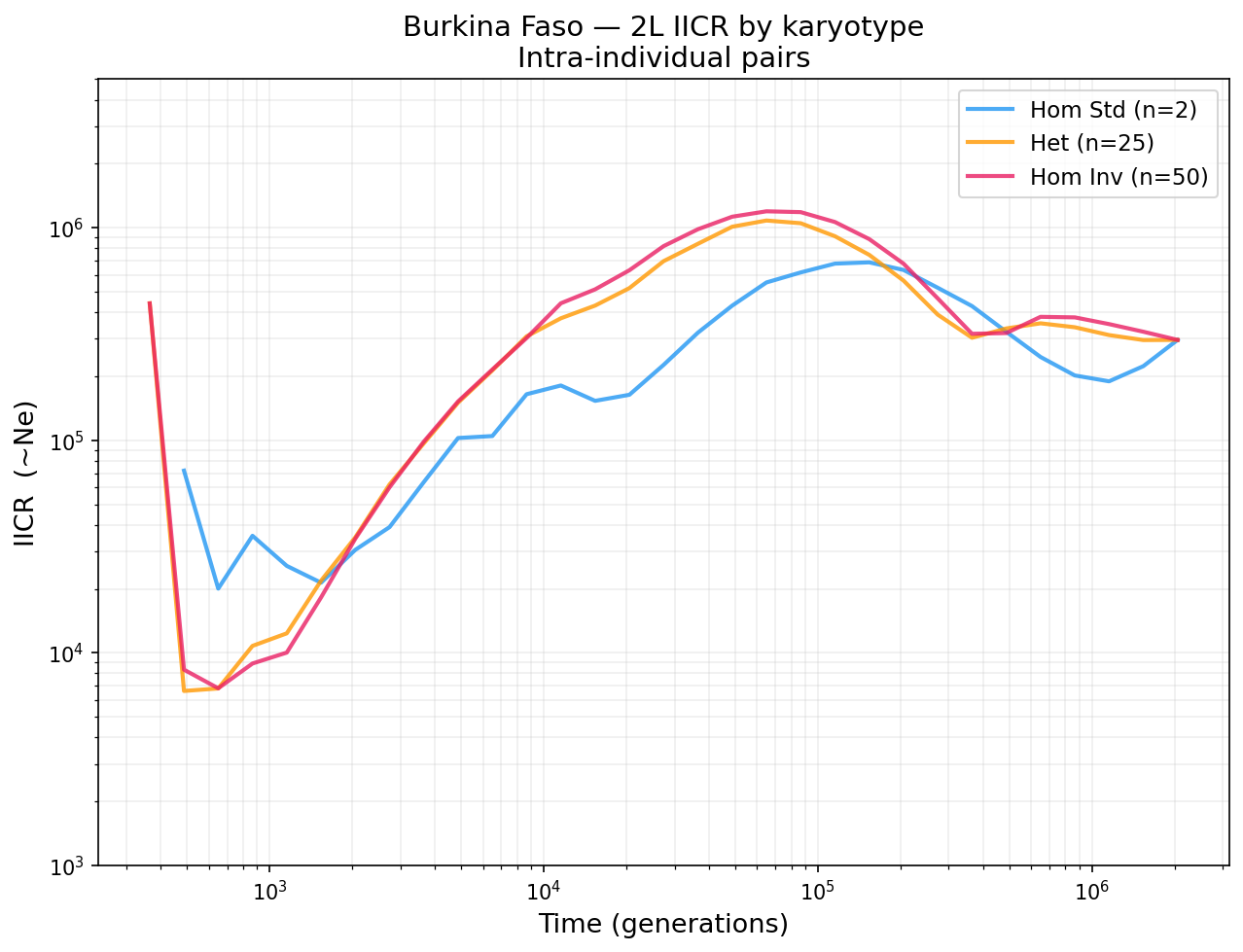
Burkina Faso 2L: heterozygous IICR (orange) shows an inflated bump at 10^4–10^5 generations from the inversion. Homozygous standard (blue) and homozygous inverted (pink) are not affected.
Best practices for demographic inference
Use 3L, 3R, or X (no known inversions) for clean demographic signals
Use homozygous karyotype groups on 2L/2R to avoid inversion artifacts
Use intra-individual pairs for IICR (both haplotypes of same individual)
Compare across multiple arms — concordance increases confidence
Always overlay the stdpopsim reference for your species