Quickstart¶

Installation¶

fastcxt requires Python 3.10+ and a CUDA-capable GPU for the Mamba kernels.

uv (recommended)

uv pip install -e ".[all]"

pip

pip install -e ".[all]"

For CPU-only development (e.g. preprocessing, simulation), install without the GPU dependencies:

uv pip install -e ".[sim,docs,dev]"

End-to-end example¶

Simulate training data with variable sample sizes:

for N in 10 25 50 100 200; do
    fastcxt-simulate --scenario constant \
        --data-dir ./sims/n${N} --num-ts 200 --n-samples $N
done

This creates 1000 tree sequences total (200 per sample size) in separate subdirectories.

Preprocess into SFS features and TMRCA targets:

fastcxt-preprocess --base-dir ./sims --out-subdir processed \
    --extract-trees --max-samples 200

The preprocessor scans sims/ recursively, discovers all .trees files, and uses each subdirectory name (n10, n25, …) as the scenario label. The --max-samples 200 flag pads tree topology features to a consistent dimension so all sample sizes can be batched together.

Train a model:

fastcxt-train --model base --dataset-path ./sims/processed --gpus 0

Run inference from Python:

import fastcxt
from fastcxt.config import PRESETS
from fastcxt.model import FastCxtModel

config = PRESETS["base"]
model = FastCxtModel(config)
# model.load_state_dict(torch.load("checkpoint.pt"))

from fastcxt.translate import translate_from_ts
import tskit

ts = tskit.load("my_data.trees")
means, variances, index_map = translate_from_ts(
    ts, model,
    pivot_pairs=[(0, 1), (0, 2)],
    mutation_rate=1e-8,
    device="cuda:0",
)

Build a TimeAtlas for genome-wide results:

from fastcxt.atlas import TimeAtlas

atlas = TimeAtlas()
atlas.add_arm("2L", means, variances, pairs, window_size=2000)
atlas.save("my_atlas/")

# Query later
atlas = TimeAtlas.load("my_atlas/")
m, v = atlas.query_pair("2L", sample_a=0, sample_b=5)

Visualize with geographic context:

# Generate showcase figures with simulated placeholder data
python scripts/plot_atlas_showcase.py --outdir figures/

This generates publication-quality geographic maps, TMRCA landscapes, population heatmaps, selective sweep panels, and a composite dashboard. See Visualization for the full gallery.

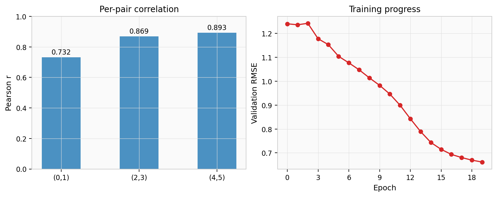
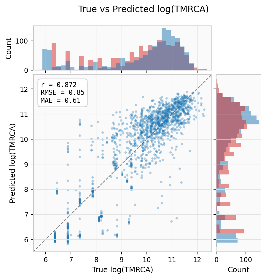
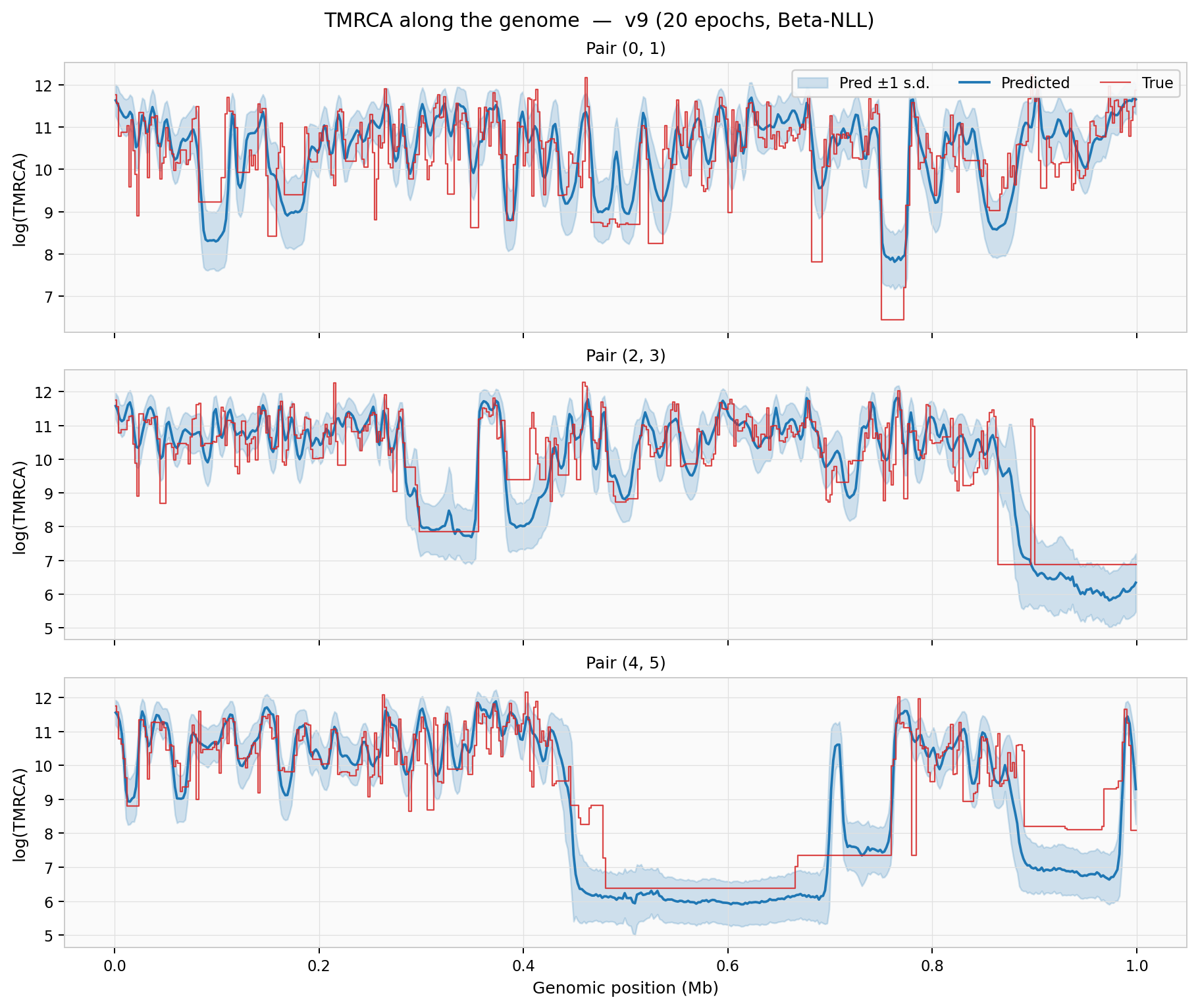
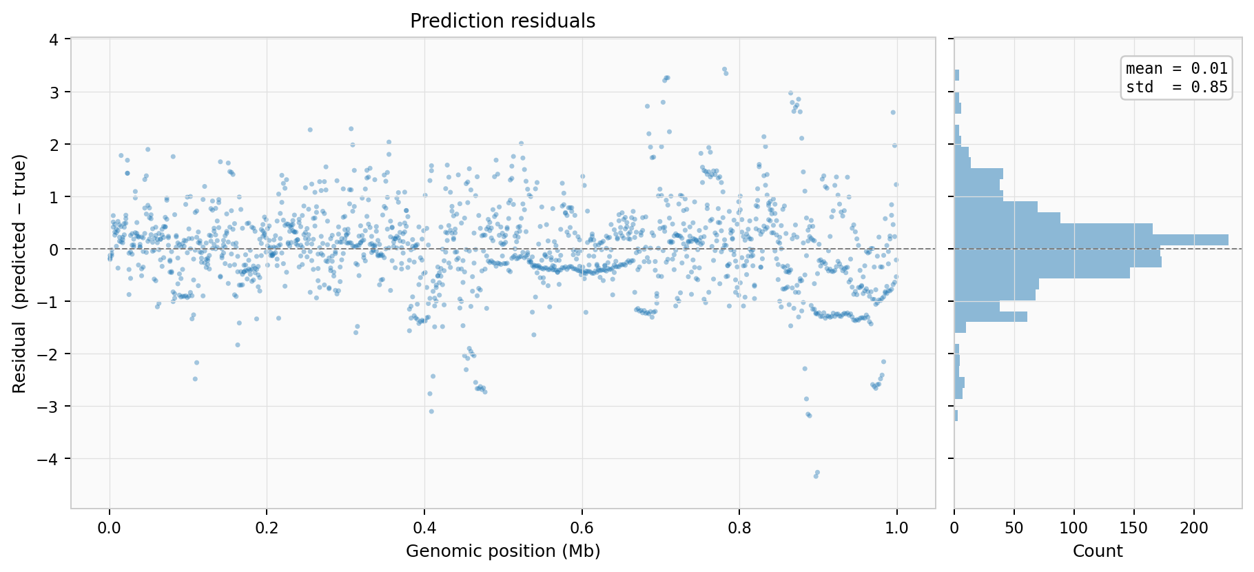
Example results¶

The figures below are from a quickstart run: 1000 constant-demography tree sequences with variable sample sizes (10–200), the base model preset trained for 20 epochs with Beta-NLL loss on 3 GPUs.

True vs Predicted log(TMRCA) — scatter with marginal histograms showing overall calibration (r = 0.87, RMSE = 0.85):

TMRCA along the genome — predicted mean (blue) with ±1 s.d. confidence band overlaid on the true values (red step) for three sample pairs:

Residuals — spatial distribution and histogram of prediction errors:

Summary — per-pair Pearson correlation and validation RMSE training curve: